Colour

David Hodge

2022-06-07

library(dplyr)
library(simplevis)
library(palmerpenguins)
set.seed(123456789)

Overview

In {simplevis}, users adhere to the following rules for adjusting colour:

• You can customise colours via the pal argument
• If colouring by a variable, use a *_col() or *_col_facet() function, and define the col_var
• If the col_var is numeric, there are continuous, bin or quantile colouring methods available
• For bin and quantile, you can modify the colour breaks using the col_breaks_n or col_cuts arguments.

In {simplevis}, there is one colour concept, which generally includes all aspects of features that is relevant to the visualisation family type. This is a consistent method across all functions, which is intended to simplify colouring.

Customise colours via the pal argument

Default palettes can be changed by providing a character vector of hex codes to the pal argument.

gg_point(penguins, 
         x_var = bill_length_mm, 
         y_var = body_mass_g, 
         pal = "#da3490")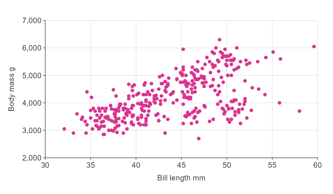

gg_point_col(penguins, 
             x_var = bill_length_mm, 
             y_var = body_mass_g, 
             col_var = species, 
             pal = c("#da3490", "#9089fa", "#47e26f"))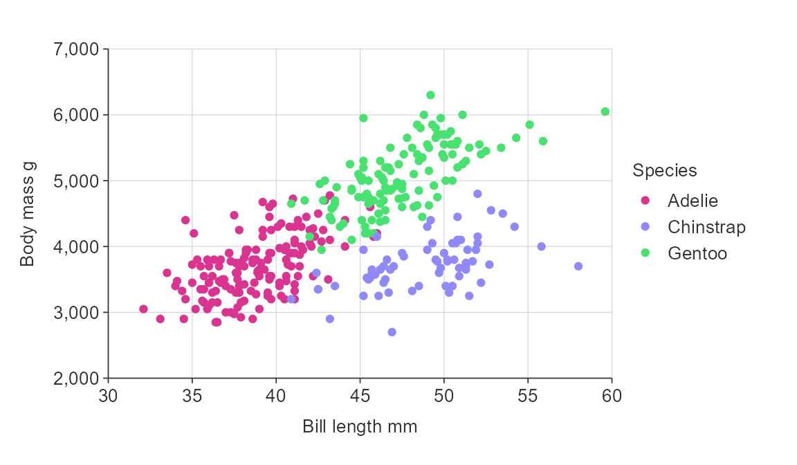

Users can get access to a large amount of colour palettes through the pals package.

gg_point_col(penguins, 
             x_var = bill_length_mm, 
             y_var = body_mass_g, 
             col_var = species, 
             pal = pals::brewer.dark2(3))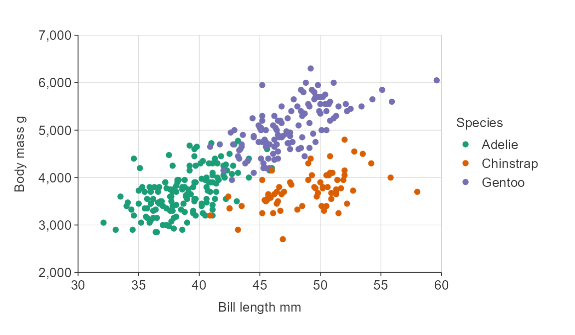

If colouring by a variable, use a *_col() or *_col_facet() function, and define the col_var

To colour by a variable, use a *_col() function and then define that variable to be coloured using the col_var argument.

gg_point_col(penguins, 
             x_var = bill_length_mm, 
             y_var = body_mass_g, 
             col_var = species)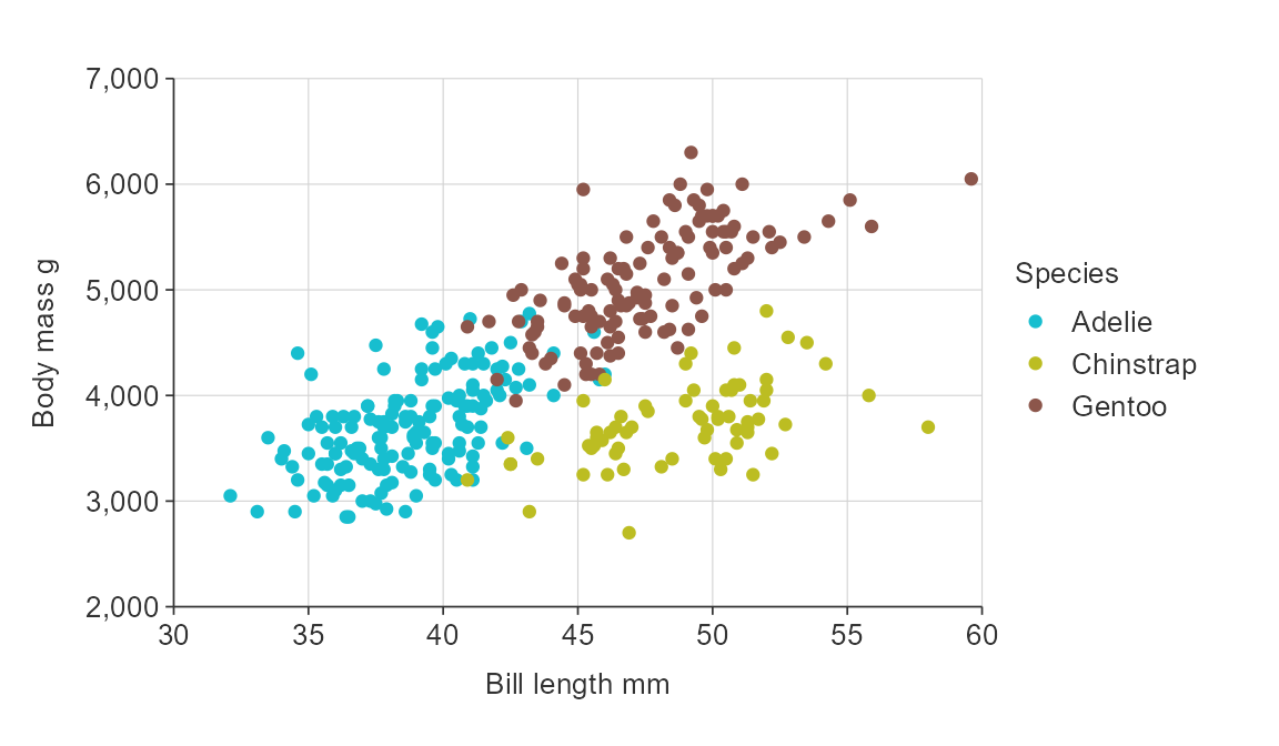

gg_point_col_facet(penguins, 
                   x_var = bill_length_mm, 
                   y_var = body_mass_g, 
                   col_var = sex, 
                   facet_var = species,
                   col_na_rm = TRUE)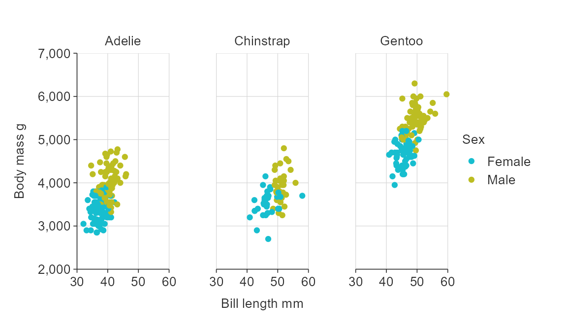

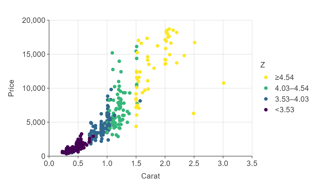
If colouring by a numeric variable, continuous, bin and quantile methods are available

All {simplevis} *_col() and *_col_facet() functions support colouring by a categorical variable.

In addition, point, bar, hbar, tile, sf and stars *_col() and *_col_facet() functions support colouring by a numeric variable.

You do this by specifying whether you want to do this by defining whether the col_method is to be by continuous (the default), bin or quantile.

plot_data <- ggplot2::diamonds %>% 
  slice_sample(prop = 0.01)

gg_point_col(plot_data, 
             x_var = carat, 
             y_var = price, 
             col_var = z)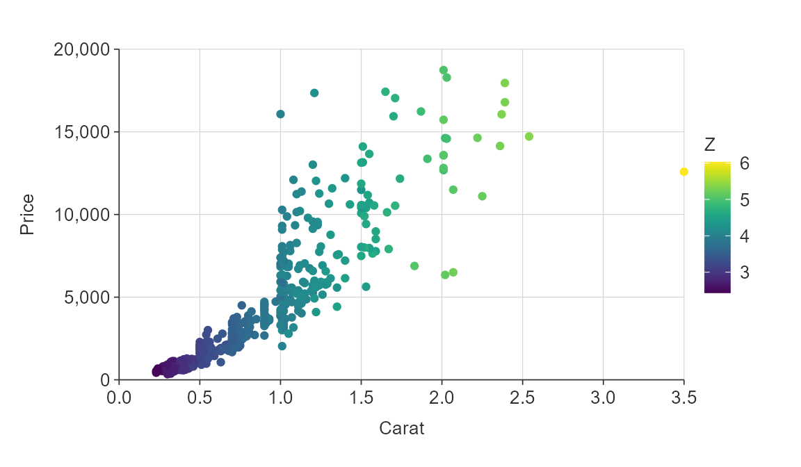

plot_data <- ggplot2::diamonds %>% 
  slice_sample(prop = 0.01)

gg_point_col(plot_data, 
             x_var = carat, 
             y_var = price, 
             col_var = z,
             col_method = "bin")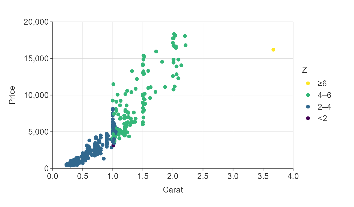

plot_data <- ggplot2::diamonds %>% 
  slice_sample(prop = 0.01)

gg_point_col(plot_data, 
             x_var = carat, 
             y_var = price, 
             col_var = z,
             col_method = "quantile",
             pal = pals::brewer.reds(4))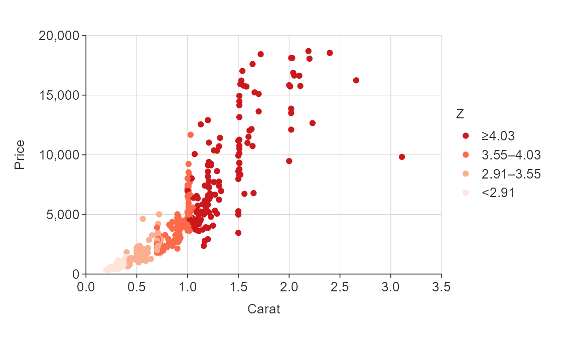

For bin and quantile, modify colour breaks using the col_breaks_n or col_cuts arguments

For bin, the col_breaks_n argument uses the pretty algorithm to aim for roughly the specified number of pretty breaks. For quantile, it selects that number of bins of equal percentiles.

Alternatively, you can specify the exact breaks you would like by specifying a vector to the col_cuts argument. For bin, this is a vector of values that should start at either -Inf or 0 and finish at Inf. For quantile, this is a vector of probabilities between 0 and 1.

gg_point_col(penguins, 
             x_var = bill_length_mm, 
             y_var = body_mass_g, 
             col_var = flipper_length_mm, 
             col_method = "bin",
             col_breaks_n = 10)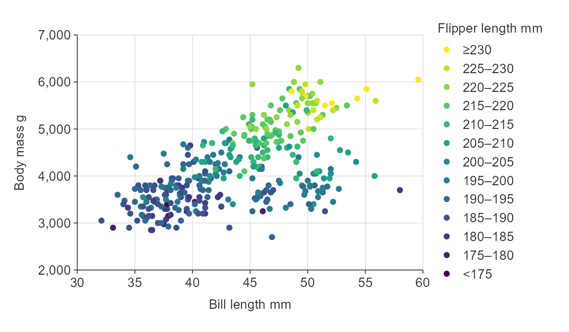

plot_data <- ggplot2::diamonds %>% 
  slice_sample(prop = 0.02)

gg_point_col(plot_data, 
             x_var = carat, 
             y_var = price, 
             col_var = z,
             col_method = "bin",
             col_cuts = c(0, 3, 4, Inf))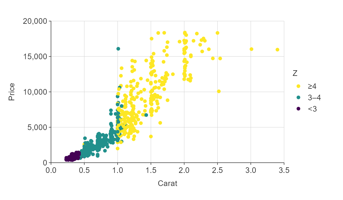

gg_point_col(penguins, 
             x_var = bill_length_mm, 
             y_var = body_mass_g, 
             col_var = flipper_length_mm, 
             col_method = "quantile",
             col_breaks_n = 8)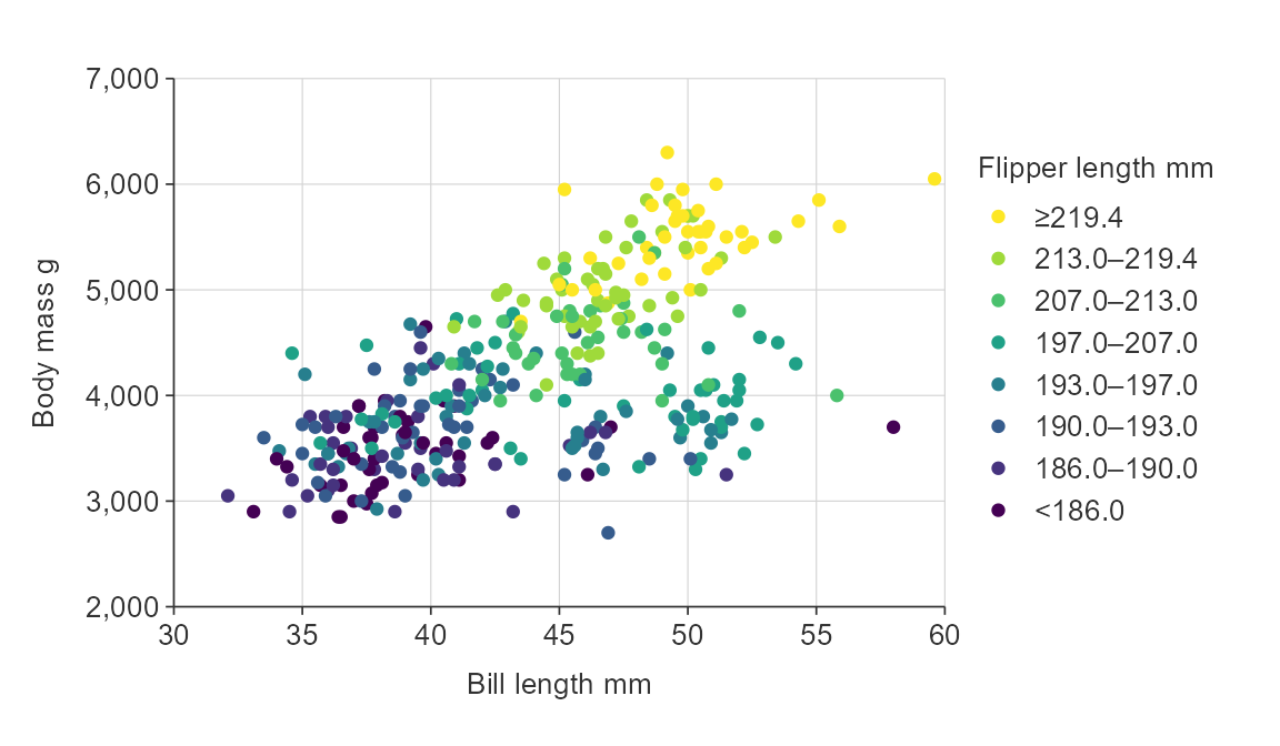

plot_data <- ggplot2::diamonds %>% 
  slice_sample(prop = 0.01)

gg_point_col(plot_data, 
             x_var = carat, 
             y_var = price, 
             col_var = z,
             col_method = "quantile",
             col_cuts = c(0, 0.5, 0.75, 0.9, 1))